November 2022

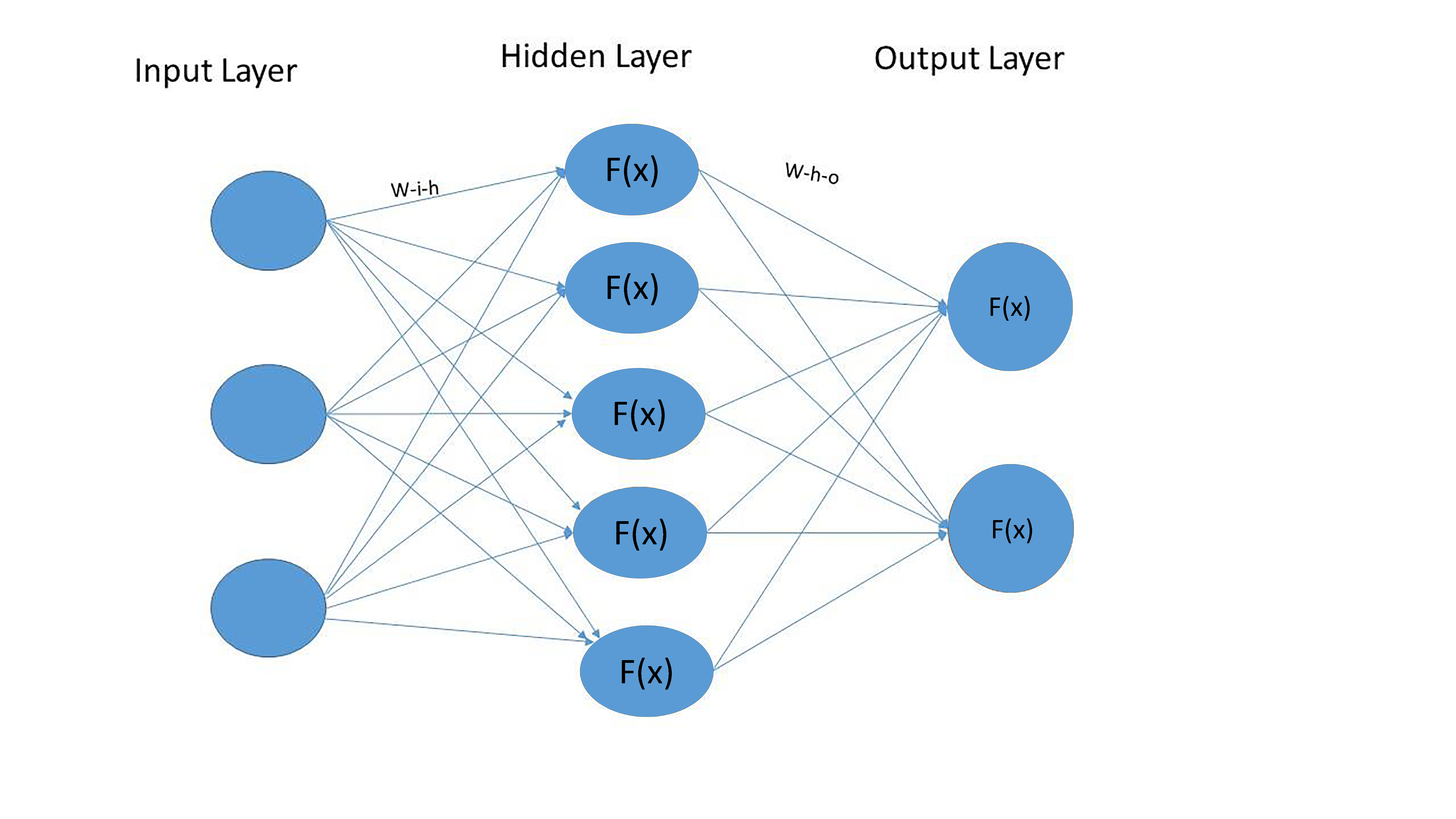
In a recurrent neural network (RNN), the hidden layer is a layer of neurons that maintains a state vector. The state vector is a representation of the internal state of the RNN at a particular timestep. The hidden layer is important because it allows the RNN to model temporal dependencies; that is, it allows the RNN to remember information about what has happened in the past and use that information to influence what happens in the future. The gradient of the hidden layer is a measure of how the hidden layer’s state vector changes over time. In other words, it is a measure of how the hidden layer learns. The gradient can be used to improve the performance of the RNN by making the hidden layer more efficient at learning. There are several ways to check the gradient of the hidden layer in an RNN. One way is to use the backpropagation algorithm. The backpropagation algorithm is a method of computing the gradient of a function by reverse-mode differentiation. Backpropagation is typically used to train neural networks, but it can also be used to compute the gradient of the hidden layer in an RNN. Another way to check the gradient of the hidden layer is to use the forward-mode differentiation. Forward-mode differentiation is a method of computing the gradient of a function by forward-mode differentiation. Forward-mode differentiation is typically used to compute the gradient of the output layer in a neural network, but it can also be used to compute the gradient of the hidden layer in an RNN. The gradient of the hidden layer can also be checked numerically. This can be done by perturbing the hidden layer’s state vector and observing how the output of the RNN changes. This method is typically used for debugging purposes, but it can also be used to check the gradient of the hidden layer.

To compute the gradient, a tensor must have its parameters requires_grad =. Partial derivatives and gradient varieties are the same. In the following example, a function for y = 2*x is used. The required_grad of the tensor – 1 is also known as the required_grad of the tensor – X. The gradient can be computed using y.

How Do You Avoid Exploding Gradients In Pytorch?

It is generally possible to avoid exploding gradient explosions by carefully configuring the network model, such as using a small learning rate, scaling the target variables, and using a standard loss function. The problem may still exist in recurrent networks with a high volume of input time steps, where exploding gradient can occur.

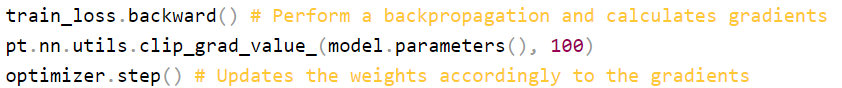
In neural networks, clipping gradient layers is a way to prevent gradient explosions. When the gradient becomes too large, an unstable network is formed. Because of the small size of the gradient, optimization encounters wobble gradient when it gets stuck at a certain point. A gradient clipping method is one of many methods of calculating it; however, it is more common to scale gradients to the value at which they function. To keep the gradient within a specified range, use torch.nn.clip_grad_norm. Clip-by-norm can be set using standard values found in literature, or using common vector norms or ranges discovered through experimentation and then selecting a reasonable value. As if they were concatenated into a single vector, all gradients are computed into a standard norm.

After that, we’ll create a collection of images and use the numpy library to load them into memory. In this case, we’ll use the torch function grad to calculate the gradient of the object we’ve created, MPoL, as well as the regularizer strength. Finally, we’ll use the numpy library’s optimize method to find the best regularizer for our datasets. PyTorch is a powerful computer program that computes the gradient of a function for use with inputs. The method is used to calculate the gradient of inputs based on a computational graph. An automatic differentiation can be performed in both forward and reverse modes. When the inputs are taken into account, the gradient of the function is computed as the function’s derivative. When the function’s gradient is compared to the inputs, the function’s integral is computed in reverse. The MPoL library is a Python library that computes the best image in a dataset using a gradient descent optimization method and randomization. The first step in the tutorial will be to import the torch and numpy packages. In this step, we will use the numpy library to generate an image dataset and store it in memory.

Gradient Clipping: A Popular Technique To Mitigate The Exploding Gradients Problem

Gradient clipping is a widely used method to reduce the gradient explosion in deep neural networks. Every component of the gradient vector has been assigned a value between – 1.0 and – 1.0 in this optimizer. As a result, even if the loss landscape of the model is irregular, the gradient descent is likely to behave reasonably, most likely to cliff. Clipping gradient ensures that the gradient vector has no abnormal behavior and can be distributed at most as close as possible to the threshold, which helps gradient descent to have reasonable behavior. LSTMt do not solve the problem of exploding gradient, but clipping gradient ensures that gradient vector has no abnormal behavior.

What Is Ctx In Pytorch?

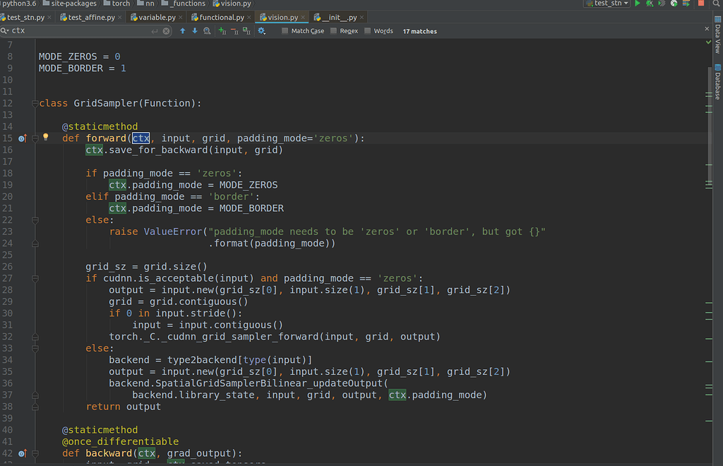
The ctx variable in pytorch is used to store the context of an object. This is useful when you want to keep track of an object’s state across multiple calls to a function. For example, if you have a list of objects and you want to keep track of the index of the object that is currently being processed, you can use the ctx variable to store the index.

Backward Pass In Neural Networks

In the backward pass, all tensor gradient distributions within the graph are computed, but the operation is only recorded if one of its input tensors requires grad.

Pytorch Get Gradient Of Intermediate Layer

To get the gradient of an intermediate layer in Pytorch, you need to first register the layer with the module so that it becomes part of the computational graph. Once the layer is registered, you can then get the gradient by calling the .grad_fn attribute on the layer.

What Does Backward Do In Pytorch?

It computes the gradient of current Tensor w.r.t. using the Tensor Principle. This graph does not leave a mark. The chain rule is used to distinguish a graph. The function will also need to specify the gradient if the tensor is non-scalar (i.e. there are more than one element in the data).

Regularization In Pytorch

In the coming sections, we’ll look at how gradient descent can be used to optimize a function if the dataset is given, as well as the desired regularization of the function. In addition, we will look at some of PyTorch’s most common optimization strategies.

What Are Hooks In Pytorch?

Each Tensor or nn has its own PyTorch hook. Modules are triggered either forward or backward by a forward or backward pass of the module object. These hooks, according to function signatures, can modify input, output, or internal module parameters. They are commonly used for debugging purposes as well as other types of analysis.

Why Pytorch Is More Pythonic

Despite its name, PyTorch feels more like a Python application than a Java application.
Its CPU-based version is one of the most popular libraries for math and data science. PyTorch, like Numpy, runs on a GPU and can perform differentiation automatically. Using PyTorch will be a breeze if you’re familiar with numpy.
Because PyTorch is more pythonic than NumPy, it was designed to be more intuitive and similar to Python. Python developers can get started with PyTorch in a hurry. PyTorch can run on the GPU, which can also be useful for certain tasks.

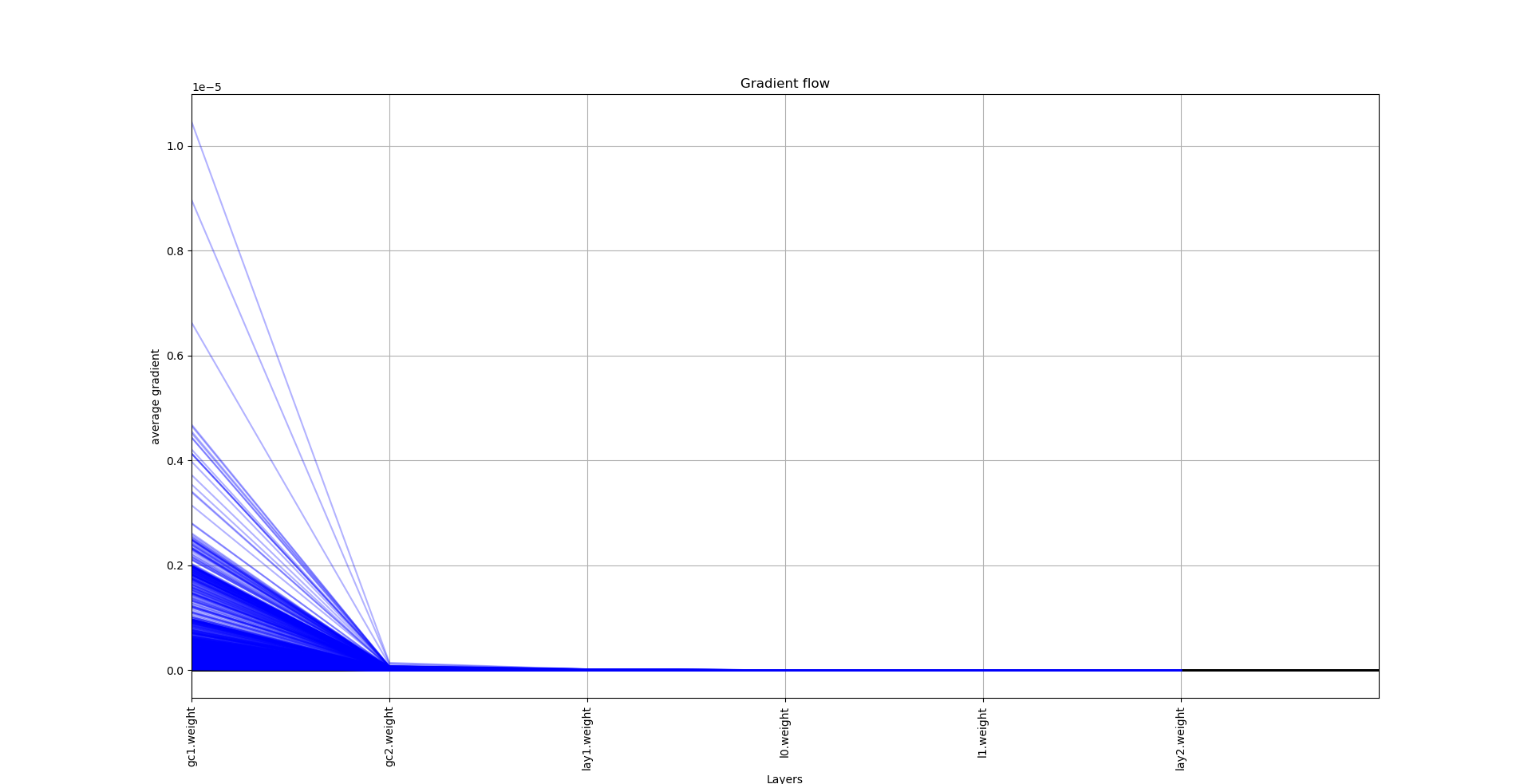
Pytorch Check Gradient Flow

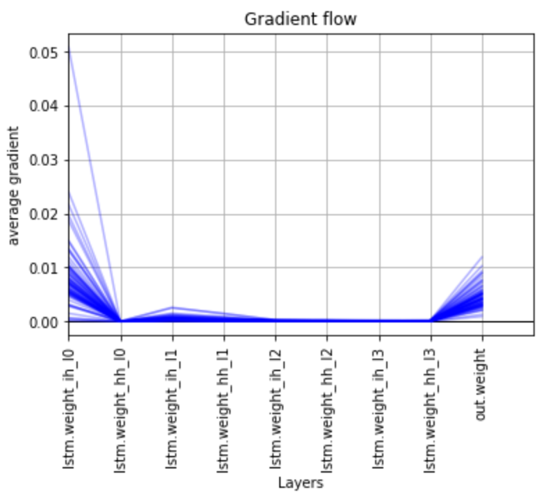
Pytorch is a popular open-source machine learning library used for both research and production. One of its key features is the ability to check the gradient flow during training. This can be useful for debugging purposes, or for understanding how the training is progressing. To check the gradient flow in Pytorch, simply call the .grad_flow() method on the relevant tensor.

Pytorch Apply Gradient

Pytorch applies gradient descent to optimize the weights of the neural network. The algorithm starts with a set of initial weights and iteratively adjusts them to minimize the loss function.

This is the PyTorch 1.13 code documentation. A function’s gradient can be calculated by including the dimensionsmathbbR*n in one or more dimensions. This gradient can be calculated by estimating each partial derivative of gg with independent precision. In practice, it is true if gg is in C3C*3 (it has at least three continuous derivatives). If the input tensor’s indices are different than the sample coordinates, spacing can be used to modify them. In this example, if spacing=2, the indices (1, 2, 3) become coordinates (2, -2, 9). If spacing is a list of one-dimensional tensors, each tensor specifies the coordinates for the corresponding dimension.

Pytorch Rnn Example

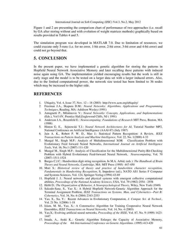
RNNs are a type of neural network that are able to processsequences of data, such as text, audio, or time series data. PyTorch is a deep learning framework that provides a way to implement RNNs in Python. This PyTorch tutorial will show you how to create an RNN that can process text, and how to train it on a dataset.

This blog post will walk you through the various types of RNN operations within PyTorch. Vanilla RNNs are typically used in conjunction with sequential data sources such as time series or natural language processing. In bidirectional RNNs, 1 RNN is fed into the input sequence, and the other RNN reverses the order. The num_layers= 3 result will result in 3 RNN layers stacked on top of each other. We obtain values from all four batches where time-steps (seq_len) equal 5 and the number of predictions equal 2 in the out. Every batch is expected to produce two outputs. If the file size is 4, 5, 2, the grad_fn=TransposeBackward1 indicates the file size.

A torch has been concealed. The torch is lit. The product measures 0.2184 in x 0.9387 in x 0,002.5 in. [ 8], [9], [10.]], [ 11,] [12, [13], [4,], [15.]], [ 16], [17], [18], [19], [20], [22.]], [ 32.

Because we set the BATCH_SIZE = 4, we produce four batches of the product. Each batch contains five rows, which is because SEQ_LENGTH = 5 in each row. We get values from all four batches where the number of time-step (seq_len) is 5 and the number of predictions is 2, all of which have a time-step of 5. Because it is both bifunctional and adaptive, it can operate both as a RNN and as a non-RNN. There are two sets of predictions. ( batch, seq_len, num_directions, hidden_size) has the second dimension, which is Grad_fn=>SliceBackward%27 (batch, seq_len, num_directions, hidden_size). To achieve forward and backward output, use a torch. ( -4, 5, 2). [ 0.0101, -0.4025], [_SliceForward, ‘SliceMidwifery,’ [_SliceLeft, ‘SliceMiddlewyth,”sliceWyth,’]: Bottom.

How To Train An Rnn With Pytorch

The goal of recurrent neural networks (RNNs) is to be able to predict the future by repeating past values. PyTorch is a valuable tool for training RNNs. In this article, I’ll go over what you need to know about RNN training with PyTorch. We’ll start with a CUDA (GPU) device for training, which is far too long to use with a CPU (the Google CoLab notebook can be used if you don’t have one). We then set the batch size (the number of elements to see before updating the model), the learning rate for the optimizer, and the number of epochs. For example, an RNN can generate a size (seq_len, batch, num_directions, and hidden_size) using batch and num_directions. In batch_first = True, the output size is (batch, seq_len, num_directions * hidden_size). The LSTMt model is used to solve the RNN’s vanishing gradient or long-term dependence issue. Gradient vanishing refers to the loss of information in a neural network over time as connections to it continue to recur. The goal of LSTMs is to reduce the vanishing gradient by ignoring useless data and information in the network.

Pytorch Visualize Gradients

In PyTorch, visualizing gradients can be done with a few lines of code. First, we need to import the necessary packages: import torch import matplotlib.pyplot as plt Then, we can define a function that takes in an input image and outputs the gradient values for that image: def get_gradient(image): # Get the gradient values for an input image gradient = torch.autograd.grad(outputs=image, inputs=torch.tensor([1.0, 2.0, 3.0], requires_grad=True), grad_outputs=torch.ones(image.size()))[0] return gradient Finally, we can use this function to visualize the gradients for an input image: # Load in an image image = plt.imread(‘my_image.jpg’) # Get the gradient values gradient = get_gradient(image) # Visualize the gradients plt.imshow(gradient) plt.show()

It is possible to perform the same operation using PyTorch in addition to the gather and squeeze methods. We can generate a network image of the target class by starting with a random noise image and performing gradient ascent on the target class. The documentation for the gather and squeeze methods can also be found here. A convolutional network can use $I$ as its image, and $y$ as its target class. To generate an image with a high Y# class score, we need to generate $I**$. We’ll show you how to use (explicitly) L2 regularization to make the form $$ R(I) = $0.0251. You can increase the number of characters by blurring the image several times.

A convolutional neural network (CNN) is a type of neural network that is typically used to analyze images. CNNs are similar to traditional neural networks in that they are composed of a series of hidden layers, but they also have a special property: they are translational invariant, meaning that they can recognize patterns anywhere in an image. This makes them especially well-suited for image recognition tasks. There are a number of different math fields that are used in CNNs, including linear algebra, calculus, and probability theory. Linear algebra is used for vector operations, such as matrix multiplication, which is necessary for performing the convolution operation. Calculus is used for optimizing the network, such as finding the gradient of the error function. Probability theory is used for modeling the distribution of data, which is important for understanding how the network will generalize to new data.

Previously, things such as computers and computers that weren’t possible were considered impossible thanks to Computer Vision. The most significant and widespread success is thought to be the contribution ofvolutional neural networks. In this article, I focus on things that most people know about CNNs. I encourage you to look at my other posts if you want more information on deep neural networks. If we scale down our photos, we will lose valuable information. The amount of data we need to use should be calculated in a clever manner, but the number of necessary calculations and parameters should be reduced. CNN is involved during this time period.

Convolution shrinks our image by half every time we perform it. Because there are only 16 unique positions where we can insert our filter into this image, we are limited in how we can apply it. Our image can be framed with an additional border to solve both of these issues. It makes no difference whether padding is used in this case; both Valid and Same convolutions are used. In this article, we will learn how to construct a single layer of CNN using convolution. Convolution is a method of image processing that is used in densely connected neural networks. When we apply multiple filters to the same image, we stack them one on top of the other.

The task of our team is to calculate derivatives associated with parameters of current layer as well as dA[l -1] – which will be passed over to the previous layer. In the following step, we will attempt to assess the impact of changing parameters on the resulting features map. Tensor dimensions such as dW, W, db, b, and dA are the same for all tensors. The first step is to use the derivative of the activation function in our input tensor to compute the intermediate value of dZ[l]. This operation will be used in the future in accordance with the chain rule. Backward propagation of the convolution will necessitate a new procedure. To accomplish this, we’ll use the full convolution matrix operation, which can be found in the image below.

In this article, we will only talk about the maximum amount of backpropagation, but the rules that we will learn apply to any type of pooling layer. There are no parameters required for this type of classification; we simply need to distribute gradiwents appropriately, so we do not need to update any parameters. Each channel in a multi-channel image must be separately assigned a pool.

One of the most important components of mathematics is linear algebra. If you only want to be a researcher and not a deep learning practitioner, you’ll need Linear Algebra even if you only want to practice deep learning. In other words, your data will be made up of multiple-dimensional matrices.

What Math Is Needed For Neural Networks?

In neural networks, linear algebra is also used to represent and process networks. As a result, if you want to work in data science, you must be familiar with linear algebra.

I started learning neural networks a few months back. The ability to comprehend neural networks’ math is extremely important in terms of understanding how they work. The next section of this article will explain the various components of a basic neural network, as well as the concepts required, as well as videos explaining the concepts. The input layer is typically represented as a vector of numbers. Because the image contains only RGB values, we can simply flatten or roll out the matrix of values in the image. The resources below will go over vectors and matrices, two concepts that must be understood as the first step in understanding neural networks. The weighted sum calculation takes into account the weight matrix and the bias.

Back propagation can actually be useful for adjusting the weights and bias in our algorithm in order to make it more accurate. You can calculate your costs using different neural networks because different neural networks use different cost functions. Our cost function can assist us in finding parameters that reduce our costs, which can be used to make our algorithm more precise. A step known as gradient descent is used to reduce costs. In order to be able to calculate the slope of a function, it is critical to understand derivatives and the method of calculating its slope. You will learn how to understand gradient descent by studying the derivatives listed below.

NNNs are nothing more than a collection of mathematical computations. Each synapsis holds a weight, whereas each neuron computes a weighted sum by using input data and synapse weights. We show that neural networks that have been trained on text and tuned to code can solve math course problems, explain solutions, and generate new questions in real time.

Why A Strong Foundation In Mathematics Is Essential For Machine Learning And Ai Developers

Math is used by researchers in the field of data science, machine learning, and artificial intelligence (AI). These professionals would be unable to implement Machine Learning and Artificial Intelligence if they did not have a basic understanding of mathematics. These four key ideas -statistics, linear algebra, probability theory, and calculus – provide the foundation for machine learning. The topics discussed here are critical to the understanding of gradient descent, backpropagation, and other algorithms used in deep learning. Deep learning networks would be difficult to train effectively if mathematics were not as strong a foundation as it needs to be. It is beneficial to understand calculus concepts before attempting to use machine learning algorithms. Although you do not need to be an expert in calculus to begin using machine learning algorithms, you should be familiar with them. Many machine learning algorithms, including those based on derivatives and integrals, are designed with calculus in mind. Derivations, for example, can be used to minimize the error in a Neural Network, which is represented by the gradient descent algorithm. If you want to work on artificial intelligence and machine learning projects, you must have a solid understanding of mathematics. Machine learning, on the other hand, requires no prior knowledge of math. Learning calculus requires a little effort, but it can be used to improve one’s AI and data science skills.

Which Algorithm Is Used In Convolutional Neural Network?

A convolutional neural network is a type of artificial neural network that is used to process images. It is made up of a series of layers, each of which contains a series of neurons. The first layer is the input layer, which is where the image is fed into the network. The second layer is the convolution layer, which is where the network learns to identify patterns in the image. The third layer is the pooling layer, which is where the network learns to identify the most important features in the image. The fourth layer is the output layer, which is where the image is classified.

Advantages Of Cnns

How does CNN algorithm work? As a result of its rectifier, the CNN network employs a ReLU layer to run elements. As a result, there is a rectified feature map. Because its built-in convolutional layer reduces the high dimensionality of images without losing their data, a CNN is the ideal machine for image and speech recognition. As a result, CNNs are especially well suited to this situation. Is CNN using SIRVAs? CNN and SVM can both be used as feature extractors in the proposed hybrid model. The MNIST dataset of handwritten digits is used to train and test the proposed model’s algorithm. CNN, in comparison to its predecessors, is able to detect critical features automatically without the use of human supervision. Because there are so many images of cats and dogs, it can learn the key features of each class on its own.

What Is Cnn Math?

CNN math is a branch of mathematics that deals with the study of neural networks and their applications in computer science. Neural networks are a type of artificial intelligence that are used to simulate the workings of the human brain. CNN math is used to develop and improve the performance of neural networks.

CNN’s Convolution Neural Network is the foundation for MATHS (Monitored Applied Technology for Human Understanding). We’ll look at CNN’s importance, as well as its math, in this topic. CNN employs a different method of detecting patterns than MLP because CNN employs layers that are not fully connected. CNN can be used for a wide range of purposes, including image recognition and video analysis. A 5X5 image size and three filters (due to each filter being used for a specific color channel: RGB) of 3X3 size. Filters are used to detect patterns and features in images. In some cases, the filter does not fit the input image perfectly.

The image must then be padred with zeros, as shown in the image below. Non-linearity is added to the convolutional network as part of ReLu. rectified linear units output no output. The raw output will be less than 0 if the input is less than zero. It is the final step in flattening our matrix and feeding its values to the layers that have been connected. The only thing I want you to understand is that this is all about CNN.

Uses For Cnns In Computer Vision

What is cnn used for?
CNNs are used in computer vision to detect objects, recognize faces, and recognize scenes.

Is Cnn A Mathematical Model?

A mathematical model is a system of mathematical equations that describes a phenomenon. CNN is a mathematical model that describes the behavior of neurons in the brain.

Cnn Can Recognize Objects In An Image Or Video

CNN can detect objects in an image or a video by analyzing the pixels in a specific area of the image. The basic idea behind it is to create a small area of an image and then divide it into smaller regions.

Types Of Convolutional Neural Networks

Convolutional neural networks are divided into three types: convolutional layers, pooling layers, and fully connected layers.

ImageNet is a large, organized visual image database that can be used by researchers and developers to train their models. In addition to the ImageNet Large Scale Visual Recognition Challenge (ILSVRC), which is a large-scale competition for object detection and image classification, they host a variety of other competitions. This list contains a collection of CNN architectures, each with a distinct design, which have been used in a variety of tasks to excellent effect. There are a lot of filters in the network, as in the original LeNet architecture, but there are also very few similarities between it and the LeNet architecture. This network is made up of 62.3 million parameters and necessitates the computation of billions of units of computation. VGGNet 16 was a runner-up to ILSVRC 2014 and was created by Simonyan and Zisserman. The GoogleNet (also known as the Inception Network) won the ILSVRC 2014 competition with a top-5 error rate of 6.67%, which was nearly the same as what human level performance would be.

Google contributed to the development of the model, which employs a more efficient implementation of the original LeNet architecture. The concept of inception is used in this way. The term ‘inception’ refers to a stack of ‘inception blocks,’ each of which contains a Max-Pooling Layer that can change the dimensions of an image. Following the completion of the network layer, a softmax regression is performed to classify the output layer, which is fully connected. It employs skip-connections and batch-normalization in its training to effectively train over thousands of layers. The 1001 layer deep ResNet performed at a top-5 error rate of 3.57%, beating the average performance of human -level datasets. It was awarded three awards at the ILSVRC 2015 in the fields of classification, detection, and localization. It was supposed to be understood that deeper layers should not make more training mistakes than shallower layers.

How Many Models Are There In Cnn?

A Convolutional Neural Network Model That Can Classify Your Fashion Images is one of the four models discussed in The 4 Convolutional Neural Network Models That Can Classify Your Fashion Images, by James Le.

Is Resnet A Type Of Cnn?

ResNet (Residual Network) is a CNN architecture that overcomes the “vanishing gradient” problem, allowing for the construction of networks with up to thousands of layers, allowing them to outperform shallower networks.

Deep neural networks are powerful machine learning models that can learn complex patterns in data. A key part of these models is the ability to learn multiple layers of representation, each of which can capture different types of information. One of the key questions in deep learning is how these different layers of representation are related to each other. In particular, do eigenvectors map each layer of a deep neural network? Eigenvectors are a type of mathematical object that can be used to represent a linear transformation. In particular, they can be used to represent the mapping between two vector spaces. Deep neural networks can be thought of as a mapping from an input space to an output space. Each layer of the network can be thought of as a transformation of the input space. The question of whether eigenvectors map each layer of a deep neural network is an important one, as it can help us understand how the different layers of representation are related to each other. There are a few different ways to think about this question. One way is to consider the eigenvectors of the transformation matrices that define the mapping between the input space and the output space. Another way is to consider the eigenvectors of the input space and the output space themselves. In general, the answer to the question of whether eigenvectors map each layer of a deep neural network is yes. However, there are some caveats to this answer. First, it is important to note that the eigenvectors of the input space and the output space may not be the same. This is because the input space and the output space may have different dimensions. Second, the eigenvectors of the transformation matrices may not be the same as the eigenvectors of the input space and the output space. This is because the transformation matrices may not be diagonalizable. Third, the eigenvectors of the input space and the output space may not be orthogonal to each other. This is because the input space and the output space may not be linearly independent. Fourth, the eigenvectors of the input space and the output space may not be normalized. This is because the input space and the output space may not have the same norm. In conclusion, the answer to the question of whether eigenvectors map each layer of a deep neural network

What Is A Deep Layer In Neural Network?

A deep layer in neural network is a layer that has a large number of neurons. This layer is usually located at the middle or end of the network. A deep layer allows the network to learn more complex patterns.

Deep learning has traditionally been used to study natural language processing, computer vision, and speech recognition, but it is also being used to study computers. Deep learning has recently been used to forecast financial outcomes, discover drugs, and diagnose diseases in a variety of other applications. Deep learning, which was initially proposed by a few researchers in the 1980s, is not a new technology. Deep learning has recently gained popularity due in part to the availability of massive amounts of data, which deep learning algorithms can exploit to improve their performance. Deep learning is a powerful tool for solving a wide range of problems because it can learn complex patterns. Deep learning can be used in a variety of domains, including computer vision, natural language processing and speech recognition, financial forecasting, drug discovery, and healthcare diagnosis. Deep learning can be used to solve a wide range of problems, and it is a powerful tool in its own right. Deep learning has recently grown in popularity as a result of the availability of large data sets, which deep learning algorithms can exploit to improve their performance.

What Are The Major Components Of Deep Neural Network?

A deep neural network is a neural network with a certain level of complexity, consisting of multiple hidden layers between the input and output layers. The hidden layers of a deep neural network can be composed of either artificial neurons or threshold units.

Tensor formats and data processing can be performed on a variety of different layers. Layers are similar to LEGO bricks in deep learning. In Keras, models of deep learning are built. The process involves cutting layers together with good-matching properties, which are used to transform data. It is more than just an art to choose the best network architecture. Our best practices and principles can be found in certain places. This method employs a highly precise variant of stochastic gradient descent (SGD). When a network has multiple losses, each of them is given a scalar quantity.

Three types of networks exist, each of which is distinguished by its structure. Each layer of an ANN performs a discrete operation on the input data, which is a subset of an ANN. The number of layers in an ANN is frequently determined by the number of neurons in a specific layer of the neural network. An ANN and CNN are similar structures in that they are made up of a variety of layers, but CNNs are more like a filter. Every layer in CNN processes a subset of the data input. The third type of network is a reinforcement neural network (RNN). A RNN is a type of news network that is similar to an ANN. Their structure, on the other hand, resembles that of a CNN. It is located at the bottom of the RNN and serves as a memory pool in the human brain.

What Are The Components Of Cnn?

The following are some components of a Convolutional Neural Network. Avolutional networks are made up of three layers: an input layer, an output layer, and a hidden layer. Convolutional neural networks differ from regular neural networks in that their layers are arranged in three dimensions (width, height, and depth).

Image data processing is an important and required step in order to use Pytorch. This step can be done with the help of a few tools and libraries. The most important tool for image data processing is the Python Imaging Library (PIL). Other tools that can be used for image data processing are the Python OpenCV library, the NumPy library, and the SciPy library. Each of these libraries has its own strengths and weaknesses, so it is important to choose the one that is best suited for the task at hand. Image data processing can be used for a variety of tasks, such as image classification, object detection, and image segmentation. In order to use Pytorch for these tasks, the image data must be processed and converted into a format that can be used by the Pytorch framework. The PIL library is the most popular tool for image data processing, and it can be used for a variety of tasks, such as image resizing, cropping, and flipping. The NumPy library is also popular for image data processing, and it can be used for tasks such as image filtering and image transformation. The SciPy library is also popular for image data processing, and it can be used for tasks such as image compression and image reconstruction.

How Do I Read Pytorch Images?

To read images in Pytorch, you will need to use the Image class. This class can be imported from the torchvision library. Once you have imported the Image class, you can then use the Image.open() method to open an image file.

How To Load Image Dataset In Pytorch

To load image dataset in pytorch, we need to first import the pytorch library and then use the ImageFolder dataset class. With this class, we can load images from a directory and automatically label them with the correct class.

Pytorch Image Dataset From Directory

There are a few ways to load in image data using pytorch. The most common is to use a dataloader which can be created using the ImageFolder class. This class assumes that images are organized into folders with each folder containing images of a single class. The dataloader can then be used to load in the images from a directory.

Pytorch Load Images From Folder

To load images from a folder in PyTorch, you can use the ImageFolder class. This class will automatically generate labels for the images based on their file names. You can then use a DataLoader to load the images into your PyTorch model.

Show Image From Dataloader Pytorch

Dataloader pytorch is a great tool for loading images into pytorch. It is easy to use and can be very helpful in loading images into pytorch.

Pytorch Dataloader Example

A PyTorch DataLoader is an iterator that provides access to a dataset. It allows you to iterate over the dataset in a variety of ways, including: – Batching the data – Shuffling the data – Loading the data in parallel using multiple workers A DataLoader takes a dataset and a sampler as input. The dataset is any subclass of torch.utils.data. Dataset, and the sampler is any subclass of torch.utils.data. Sampler. For example, to iterate over a dataset of images in batches of 32 using a random sampler, you would do the following: “` from torch.utils.data import DataLoader dataset = … # some dataset sampler = torch.utils.data. RandomSampler(dataset) dataloader = DataLoader(dataset, batch_size=32, sampler=sampler) for data in dataloader: # do something with the data pass “`

The Dataloader: A Convenient Way To Load Pytorch Datasets

The DataLoader allows you to load a dataset and its associated labels into a PyTorch instance in a simple and convenient manner. It can run either map-style or iterable-style datasets, and it can load single- or multi-process datasets in a variety of ways, such as by customizing the loading order and adding automatic batch (collation) and memory pinning.

Pytorch Load Dataset From Folder

To load a dataset from a folder in PyTorch, you can use the ImageFolder class. This class assumes that the images in the folder are organized into subfolders, with each subfolder containing images of the same class. The images can be in any format, but they should all be the same size.

Pytorch Data Loader Tutorial

A Pytorch data loader tutorial can be found here: https://pytorch.org/tutorials/beginner/data_loading_tutorial.html This tutorial covers how to write a custom dataset class, how to define a dataloader, and how to use the dataloader to train a model.

Pytorch Class

Pytorch class is a powerful tool for deep learning. It allows for easy and efficient training of neural networks. Pytorch class makes it possible to use all the features of Pytorch in an easy to use and convenient way.

Pytorch Is A Powerful Machine Learning Library

PyTorch is a neural network-based deep learning library that can be used to develop and train neural network-based deep learning models. PyTorch runs in both a Python and a C language. Because PyTorch runs solely in C, it provides a large codebase that includes key functionality like tensors and automatic differentiation, as well as a pure C interface to the PyTorch machine learning framework. While PyTorch is primarily based on Python, the C++ codebase sits atop a substantial Python codebase, providing an extremely robust and well-integrated interface.

A neural network is a machine learning algorithm that is used to model complex patterns in data. Neural networks are similar to other machine learning algorithms, but they are composed of a large number of interconnected processing nodes, or neurons, that can learn to recognize patterns of input data. The number of images that you need to train a neural network depends on the complexity of the patterns that you are trying to learn and the number of neurons in the network. Generally, the more complex the patterns and the more neurons in the network, the more images you will need to train the neural network.

This is not a universally accepted rule of thumb because it is highly dependent on the classification/regression problem and the nature of your images. In general, it takes thousands, but orders of magnitude are more common. A smaller example would be the LUNA16 lung nodule detection challenge, which only has about 1000 images.

A CNN algorithm with 100 images is quite small. The amount of samples needed is determined by the specific problem, and each sample should be tested individually. To make generalizations about the problem, a CNN algorithm must be trained with a large sample set, with a data set greater than 5,000 samples.

How Many Samples Do You Need To Train A Neural Network?

There is no one answer to this question as it depends on many factors, such as the size and complexity of the neural network, the type of data being used, and the desired accuracy of the results. In general, however, it is typically necessary to use a large number of training samples in order to train a neural network effectively.

As a result, this rule of thumb states that if we are attempting to predict the behavior of an unknown set of data, we need more data than we can predict. We cannot reliably determine the relationships between the variables in the new data set because we lack enough data. This rule of thumb may not always be sufficient in some cases. We can get good results in many cases when we have fewer than 1,000 samples. To make the most of our data, we can use machine learning algorithms in many cases to find hidden patterns. Machine learning has the ability to detect patterns in our data that we would otherwise be unaware of. As a result, in many cases, good predictions can be made with a small number of samples rather than a large number of samples. In other words, having data at least ten times the degree of freedom is critical to obtaining a good result.

The Power Of Computers In Neural Network Weighting.

Even with the most powerful computers, it can take weeks or even months to figure out which weights should be applied to a neural network.

How Many Images Can A Neural Network Classify?

Convolutional neural networks (CNN) are a class of deep learning neural networks. CNNs have made significant contributions to image recognition. Their primary function is to analyze visual imagery, but they are also used behind the scenes.

Layers Of A Neural Network

A combination of the input layer and the output layer is commonly referred to as an input layer. When a neural network is applied to an image, it is inputted to the input layer, which outputs the image using the input layer. There is a third layer called the convolutional layer in the above layer. This layer uses an image as input, then applies a series of convolutions to it. Convolutional images are spread across the entire neural layer’s width and height by employing a two-dimensional operation. The fourth layer is made up of the pooling layer. This layer takes a number of outputs from the previous layer and combines them into a single output. It is the fifth layer, which is completely connected to the first. The fourth layer contains more neurons than the fifth, but it is similar in structure. Finally, the sixth layer is one with a weight decay. This layer is known as the dropout layer. In the following layer, a number of previously generated outputs are discarded. When an eighth layer’s weight decays, it becomes fully connected. The dense layer is located at the ninth layer. The classifier is in the tenth layer.

How Many Images Do You Need To Train Object Detection?

Object detection is a complex task that requires a large amount of data to train. The more images you have, the better the results will be. However, you need to be careful about overfitting your data. If you have too many images, your model will start to memorize the training data and will not be able to generalize to new data.

How Many Images To Train Tensorflow

There is no definitive answer to this question as it depends on a variety of factors, including the complexity of the images and the desired accuracy of the results. A good rule of thumb is to use at least 1000 images for training, but more may be needed depending on the circumstances.

How Many Images Do I Need

The number of images you need will depend on the project you are working on. For example, if you are creating a website, you will need more images than if you are creating a presentation.

An evolving neural network is a neural network that can automatically adapt and improve its performance over time. This type of neural network is often used in applications where the data or the environment is constantly changing, such as in stock market prediction or weather forecasting. There are many different ways to program an evolving neural network. One common approach is to use a genetic algorithm. This involves using a population of neural networks, where each individual network is a potential solution to the problem. The networks are then evaluated on their performance, and the best ones are selected to be used to create the next generation of networks. This process is repeated over time, and the neural networks gradually evolve to become better at solving the problem. Another approach is to use reinforcement learning. This involves training the neural network on a series of tasks, and providing it with feedback on its performance. The network can then use this feedback to adjust its parameters and improve its performance on future tasks. Regardless of the approach used, evolving neural networks can be very effective at solving problems that are difficult for traditional neural networks. They are able to adapt and improve their performance as the data or environment changes, making them ideal for applications where the conditions are constantly changing.

This tutorial on evolutionary algorithms is intended to teach you how to develop neural networks. Algorithms are built on the premise that natural selection takes place. In this tutorial, we will use an evolutionary algorithm to train neural networks. By applying this method, we can solve regression, classification, and policy issues. You can learn more about fitness functions by looking through the applications section below. To generate a new generation of n organisms, we must take n sets of organisms from the previous generation. Each child should be assigned a fitness score based on their ability to parent, and the organism that will parent them should be determined on this basis.

When fittest organisms reproduce, they produce the most offspring. The first two steps are to add Gaussian noise to each weight in the network. The fourth step is a mutation. Each child organism is prone to mutation once it is born (snippet 3, line 18). Step 5 is repeated. Only after some conditions are met are we forced to return to step two if others are not met. Evolutionary algorithms are simple to implement and effective.

In this experiment, we’ll look at evolving organisms capable of playing OpenAI’s CartPole game. The ecosystem evolved an organism that defeated the game in only six generations. Evolutionary algorithms, in addition to their benefits for machine learning, are well worth the time and effort put in.

What Programming Language Is Used For Artificial Neural Network?

There is no one answer to this question as different programming languages can be used for artificial neural networks. Some popular choices include Python, R, and MATLAB. Each language has its own strengths and weaknesses, so it is important to choose the one that is best suited for the particular application.

Python has the flexibility and ease-of-use that make it an easy language to learn. As a result, it is an excellent tool for both novice and seasoned artificial intelligence developers. Additionally, Python comes with pre-existing libraries for AI development, making it simple to start building AI apps with Python. Python is available in a number of AI software applications. Among the most popular are Neural Designer, Neuroph, Darknet, Keras, NeuroSolutions, Tflearn, ConvNetJS, Torch, NVIDIA DIGITS, Stuttgart Neural Network Simulator, DeepPy, MLPNeuralNet, DNNGraph, and AForge. Each of these tools has its own set of features and advantages. Choosing the right tool for a job requires a good understanding of the available Python-based AI software options, which include a wide range of capabilities.

What Is The Most Advanced Neural Network?

Most advanced neural networks are those that have been designed to mimic the way the human brain learns. These networks are composed of a large number of interconnected processing nodes, or neurons, that can learn to recognize patterns of input. The most advanced neural networks are able to learn to perform complex tasks such as facial recognition, object classification, and even machine translation.

Despite the fact that artificial intelligence has been developed for many years, it is still unknown what functions the brain performs. The human brain is one of the more complex neural structures ever discovered.
GPT-3, the largest neural network ever built, can generate convincing text that looks and sounds like a human could have written it. Because the network can capture the nuances and nuances of human language, it is an excellent tool for creating AI that is more convincing and human-like.

Evolving Neural Networks With Genetic Algorithm

Evolving neural networks with genetic algorithm is a process of optimizing a neural network by using a genetic algorithm to iteratively improve the network. This process can be used to optimize the network for a specific task or for general performance.

The goal of this blog is to answer a simple question: Is it possible to train neural networks with selection and evolution observable in nature? Then, we’ll go over what evolution means and what factors must be present in order for it to simulate such an environment. The paper Evolving Neural Networks Through Augmenting Topologies will be discussed, as will a discussion of the National Evolutionary Synthesis Team (NEAT). The goal of Neural Network Analysis and Theory (NEAT) is to better understand how genetic information from parents is used to produce offspring. NEAT employs two methods of encoding genes: one for nodes and one for connections. One neural network’s genomes may be crossed over to another, resulting in an incorrect encoding that causes both networks to fail. It is used to create a 16-bit binary code-based model of how a gene’s DNA would look like if encoded in 16-bit binary code.

Two genes are instantiated into agents, each representing 8 bits of information about the genetic code. A brain is formed from these 16 bits as it traverses this graph to make decisions that will determine its behavior. We need to instantiate the agents with two genes because we are encodeing two gene pairs. As they pass their genes, they shift toward the left. In order to create more complex behaviors, the bit length and genome length of the genes could be increased.

Evolutionary Neural Network Python

There is no one-size-fits-all answer to this question, as the best evolutionary neural network for Python will depend on the specific needs and goals of the user. However, some popular options for evolutionary neural networks in Python include NEAT (NeuroEvolution of Augmenting Topologies) and PyBrain. NEAT is a well-known framework for evolving neural networks that is easy to use and provides good results. PyBrain is another popular framework that is also easy to use and provides good results.

Evolutionary artificial neural networks (EANNs) can be thought of as a sort of artificial hybrid. Evolutionary search, as well as neural networks and genetic algorithms, are examples of these. There are three levels of evolution in EANNs, i.e. the evolution of connection weights, architectures, and learning rules, according to this paper. Nonetheless, it concludes that it is still early in the process of determining how these various levels interact. Grundstrom EL and Reggia JA were awarded the Turing Award. An activation rule is learned over a connection weight. The COVID-19 contagion forecasting framework is based on evolutionary artificial neural networks and curve decomposition. Daz-Lopez M, Guijo-Rubio D, Gutiérrez PA, Gmez-Orellana AM, Tez I, Ortigosa-Moreno L, Romanos-Rodrguez A, Padillo-Ruiz J,

The Different Types Of Genetic Algorithms

GA, an extremely powerful and versatile algorithm, can be used for a variety of applications. It has been used in a variety of applications, including computer graphics, signal processing, machine learning, and artificial intelligence. A number of GA variations, including particle swarm optimization (PSO), simulated annealing (SA), and genetic programming, can be implemented. In further detail, please refer to the following table for each of these variations’ strengths and weaknesses. A particle-based approach is used in the PSO, which is a generalized architecture. This algorithm has been used to solve a variety of problems, including image processing, computer vision, and natural language processing. The simulated annealing method is used in the SA. The algorithm’s speed and tolerance for variation are both slow, but it does have a high tolerance for variation. It is used in situations where the general-account (GA) cannot be applied, such as nonlinear optimization and scheduling problems. GPs are genetic algorithm-based GAs. This algorithm has a low tolerance for variation and is fast. It can be used to solve problems that are easy to solve with general relativity, such as combinatorial optimization problems.

Tensorflow Evolutionary Neural Network

TensorFlow is an open source software library for numerical computation using data flow graphs. Nodes in the graph represent mathematical operations, while the graph edges represent the multidimensional data arrays (tensors) that flow between them. This flexible architecture lets you deploy computation to one or more CPUs or GPUs in a desktop, server, or mobile device with a single API.

The Benefits Of Neural Networks And Genetic Algorithms

*br> The following are the advantages of using Neural Networks and Genetic Algorithms. Neural Networks and Genetic Algorithms are extremely versatile and can be used in a variety of applications.
A network is a tool that can be used to solve a variety of problems, whereas genetic algorithms can be used to optimize solutions for specific problems.
The learning and improvement processes of Neural Networks and Genetic Algorithms are entirely their own.
Because neural networks and genetic algorithms can change over time, they are better able to perform the tasks they were designed to perform.

A neural network is a machine learning algorithm that is used to model complex patterns in data. Neural networks are similar to other machine learning algorithms, but they are composed of a large number of interconnected processing nodes, or neurons, that can learn to recognize patterns of input data. Neural networks are well suited for tasks that require the machine learning algorithm to learn from experience and improve its performance over time. For example, neural networks are often used for tasks such as image recognition, facial recognition, and speech recognition. To build a neural network, you need to specify the number of neurons in the input layer, the number of neurons in the hidden layer, and the number of neurons in the output layer. You also need to specify the activation function for the neurons in the hidden layer. The activation function determines how the neuron will respond to an input. There are many different types of activation functions, but the most common activation function is the sigmoid function. The sigmoid function squashes the input to a value between 0 and 1. This makes the output of the neuron easier to interpret. Once you have specified the number of neurons and the activation function, you need to initialize the weights of the connections between the neurons. The weights of the connections determine how strongly one neuron is connected to another. The next step is to train the neural network. To do this, you need to feed the neural network with training data. The training data is a set of examples that the neural network can use to learn the correct mapping from inputs to outputs. After the neural network has been trained, you can test it with new data. If the neural network is able to correctly map the inputs to the outputs, then it has learned the task.

In this tutorial, we’ll look at the canonical dataset MNIST, which contains handwritten digits, as well as a number of images. A simple neural network will be developed to classify these handwritten digits into fives, or not fives. In this case, the character is read using optical character recognition. Using Keras, we can build our model in only 30 lines. The three most effective methods for improving your model are activation, gradient descent, and mean squared error correction. activation functions convert large positive numbers into 1 large negative numbers into 0, and everything between is a value between 0 and 1. If the output is a five, it must also be a five or something else.

Is It Easy To Create A Neural Network?

No, it is not easy to create a neural network. Neural networks are complex structures that require a lot of planning and design before they can be created. The process of creating a neural network can be difficult and time-consuming, but it is possible to create one if you have the right tools and knowledge.

Understanding the inner workings of a Neural Network is critical for aspiring Data Scientists. I will be using a low-cost, open-source deep learning library, TensorFlow, in order to construct a neural network from scratch in order to gain a better understanding of Deep Learning. Please see the article for details, and if you enjoy it, please feel free to share it with others. Two layers of a simple two-layer Neural Network produce the following output: In training, one of the primary goals is to find the best set of weights and biases that minimize the loss function. This tutorial will be written using a simple sum-of-sqaures error as our loss function. Each iteration of the training process is distinguished by the following steps: It is critical for our Neural Network to master the ideal set of weights in order to represent this function. We must estimate the weights on the fly to make them work. As a result, the chain rule must be used to calculate this. To test what happens when you train the Neural Network 1500 times, we’ll take the Neural Network 1500 times.

Creating A Neural Network From Scratch

By following simple steps, it is simple to build a neural network. With the necessary data and computational power, a Python or R library can be used to generate and train a neural network with accuracy on any dataset. Furthermore, if you use a library, you can create your own neural network. In this tutorial, I will show you how to implement a neural network, forward propagation, and backward propagation without using any libraries.

Neural networks are widely used today in many different applications, from facial recognition to self-driving cars. In this tutorial series, we will be using the open source TensorFlow library to build and train our own neural networks from scratch. We will start by introducing the basics of neural networks, including their architecture and how they are trained. We will then move on to building our first neural network in TensorFlow, and training it on a simple dataset. Finally, we will explore some more advanced applications of neural networks, such as building a network to classify images. By the end of this series, you will have a good understanding of how to build and train neural networks using TensorFlow, and you will be able to apply these skills to your own projects.

How Does A Neural Network Get Trained?

A Neural Network is defined as training a Neural Network in which the appropriate Neural Connections weights are found using Gradient Backward propagation, which is a feedback loop.

The Efficientnet B0 Algorithm: How Neural Networks Learn

The text below serves as the starting point for this editorial. Neural networks can often take a long time to train, especially if you use an efficient algorithm like EfficientNet B0 for example. Because we want to avoid wasting time during training, we frequently review the network’s accuracy mid-training.
Neural networks make use of data that has been trained by following a reverse process of backpropagation. In the reverse process of propagating forward inputs, weights, and biases, the network actually learns by determining what changes to make in the weights and biases required to produce the correct results.
Data sets are commonly used to train neural networks, but neural networks must learn on their own. Network researchers then employ this knowledge to improve their predictions’ accuracy.

How Do Neural Networks Learn From Trained Data?

Neural networks learn by tweaking the weights of the connections between neurons until the output of the network closely matches the expected output for a given input. This process is known as training the network.

Neurons are made up of layers of computational units (neurons), with connections among them. The networks transform data until they can identify it as an output, such as when naming an object in an image or tagging unstructured text. Michael Skirpan used animations to illustrate how neurons learn as part of a network visualization. An emergent system is a neural network, a complex system with a variety of emergent behaviors. When neurons interact with one another rather than with the neuron itself, learning occurs. The goal of this visualization is to demonstrate how a neural network learns to find the right answer on its own by tuning itself. Neural networks are similar to brain systems in that they accept and process new information, determine the correct response to it, and reflect on the mistakes they make to improve their performance in the future. Even though we don’t know what kind of intelligence neural networks will produce in the future, we should understand how learning works so that we can better predict what will be possible in the future.

Deep Learning: The Future Of Artificial Intelligence

Deep learning has revolutionized the field of artificial intelligence, allowing machines to learn patterns and navigate complex data sets. Deep learning entails the use of neural networks, which are made up of many layers. The nodes in a node pool are responsible for training on a subset of the data, whereas the deeper the layer, the more sophisticated the data that the node can recognize.

Neural Network Tensorflow Example

A neural network is a system of hardware and software that is patterned after the operation of neurons in the human brain. Neural networks are used to recognize patterns, make predictions, and perform other tasks that are difficult for conventional computers to perform.
TensorFlow is an open-source software library for machine learning that was developed by Google. TensorFlow allows developers to create dataflow graphs, which are networks of nodes that represent the calculations that are performed on the data.
One of the most popular examples of a neural network is the Google Brain project, which used TensorFlow to create a neural network that was able to learn to recognize cats in YouTube videos.

This is one of the highlights of our TensorFlow guide. It is based on the Trip Advisor Las Vegas Strip Hotel Dataset. The authors created a model using R, and they used Support Vector Matrix (SVM) algorithms to achieve their results in their paper. TripAdvisor has compiled a list of 21 hotels along the Las Vegas Strip. In this case, the model will predict how much money an individual will give to the hotel based on their past performance. Machine learning necessitates the conversion of all of these values to integers, which is done by using arrays of numbers as input. When we’ve finished making predictions, we can use our TensorFlow Neural Network to do so.

Tensorflow’s tf.decode_csv() method can read one line at a time by providing the dataset map() method for each line. Tensors are used in Tensorflow to create a TensorFlow dataset, which is not a standard Python dataset. Tensor creation is required for each column in the dataset because we have categorical data (for example, 0 and 1) as well as numbers (for example, the number of reviews). It appears in the code’s final section, where we provide the model’s feature columns and a directory with the model’s location. In a separate blog post, we will demonstrate how to use this model to predict how a hotel will be rated based on a customer’s characteristics. As a result, the hotel could decide how much effort it would need to make this customer happy or whether it would be worthwhile.

The Benefits And Drawbacks Of Using A Multilayer Perceptron

What is a multilayer perceptron and how does it work? It is a neural network with a number of simple linear units that is referred to as a multiplexer. Linear units have weights and bias, which are used to calculate their input output. The MLP is trained in algorithm by employing gradient descent. What is the advantage of using a multilayer pulser? Several advantages of using a multilayer perceptron can be discovered. Because of its ability to detect data with high resolution, the multilayer perceptron is an excellent tool for solving complex problems. Perceptrons with multilayer properties can be used to generalize new data. Multilayer patterns are sophisticated enough for a multilayer perceptron to learn. What are the drawbacks of using multi-layered pneumatic valves? Multiple layered Perceptrons have some disadvantages. It takes a lot of computational power to design a multilayer perceptron. A significant number of training samples are required for a multilayer perceptron to work. The training of multilayer perceptrons can be difficult.

Tensorflow Training Model

TensorFlow is a powerful tool that allows developers to create and train sophisticated machine learning models. While TensorFlow can be used for a wide variety of tasks, it is most commonly used for training neural networks. Neural networks are a type of machine learning model that are designed to mimic the workings of the human brain. By training a neural network on a large dataset, it can learn to recognize patterns and make predictions. TensorFlow makes it possible to train neural networks quickly and efficiently, and has become the go-to tool for many machine learning developers.

The Tensorflow.js JavaScript library is used to train and deploy machine learning models in the browser using Tensorflow.js. A Tensor Model is made up of multiple layers, which is what makes it a neural network. When constructing a model for a Machine Learning task, you must combine different types of Layers into a model that can be trained to predict the value of future changes. The output from one layer is referred to as the input from the next layer in a sequential model. In the model, layer one is made of only one unit (tensor) and shape one is made up of one dimentional. In this example, I call a function to plot the prediction graphs based on the results of the ten-y-value prediction and ten-x-value prediction.

How To Train A Neural Network In Python Tensorflow

To train a neural network in python tensorflow, you will need to first install the required libraries. Next, you will need to load the data that you wish to train the neural network on. Once the data is loaded, you will need to define the neural network itself. Finally, you will need to train the neural network by feeding it the data and adjusting the weights accordingly.

This tutorial assumes that you have a basic understanding of neural networks, which you can learn if you need to go over them in detail in the neural networks tutorial. In this project, we will create a simple three-layer neural network to classify MNIST data. This tutorial’s code can be found in GitHub, the website’s repository for developer projects. TensorFlow aims to be a high-performance, parallel operation-based machine learning platform that can make significant performance improvements by facilitating increased efficiency. A three-layer neural network is depicted on this computational graph. At each point, relevant tensors flow to the Gradients block, which is responsible for performing back-propagation and gradient descent. The old version of TensorFlow did not support a direct look at a tensor, so you had to rely onnumpy, a library known as Numerical Python, to do so.

Tensor 2 has been introduced to improve the flow. The method numpy() – which uses the tensor’s numpy form – will be shown shortly, but the command to access the tensor’s numpy form is straightforward. The TensorBoard functionality, which is included with Tensor Flow, can be used to visualize a simple graph like this one. Using numpy, a developer can directly change the indices or slices of an array. What is the same for TensorFlow 2? Yes, but not as plainly as in numpy. The three-layer neural network demonstrated in this section is simple to implement.

Machine learning relies on a large number of basic, common image classification datasets, such as those from MNIST. Training rows, testing rows, and validation rows total 60,000 rows. The colors in these images are grayscale (i.e. black and white), indicating the intensity of the whites in each color. To increase training efficiency, the program must be scaled so that it is between 0 and 1. The length of the data being transmitted is passed to a function, which generates a random vector of integers with values ranging from 0 to 100. In other words, a batch size equal to the number of random integers generated equals a random integers generated size. The x and y data are returned, but the return data is only for those random indices that were chosen.

In the coming days, a demonstration will show how to do this on numpy array objects. Using the code below, we will look at how input data is processed by neural networks. Data is first re-typed using TensorFlow’s cast function, and then matrix-multiply into Tensors using matmul. The tensors are fed into a hidden layer of the network known as W1, where W is the weights matrix, x is the layer input vector, b is the bias, and f is the node’s activation function. The code below explains how Tensorflow’s optimizer function will be implemented in the main training loop. The average cross-entropy loss per sample must be minimized as part of the optimization process in order to train neural network weights. This is accomplished by computing the mean of the tensor supplied with the use of the tf.reduce_mean function.

It involves the evaluation of the loss function in addition to all of the variables and operations involved in feeding forward data through your network. The GradientTape API adds a new feature that allows you to specify which variables and operations you want to use to generate gradient values. When we call nn_model and loss_fn within the gradient tape context, we know exactly where the gradient of the neural network is calculated. TensorFlow maintains a track of all of the variables and operation results so that they are ready for gradient computations at all times. To complete the gradient descent step, an optimization files a zip file with the weight and bias variables before sending these gradient returns to the user. Tensor sizes can be inspected and converted to numpy arrays, operations can be performed on-the-fly, and so on with TensorFlow 2. The logits output of the model will be in the following dimensions.

To find the maximum number of columns for each of the 10 output nodes, we want the argmax function to find the maximum in each of the dimensions. In this tutorial, we’ll walk you through how to train a deep neural network using TensorFlow. This code produces a list of output items, which include epoch number, average loss, and test set accuracy. When the average loss decreases on an average after each epoch, something is wrong with the network or the learning has stalled.

Neural Network Using Tensorflow

A neural network is a computer system that is modeled after the brain. It is composed of a series of interconnected processing nodes, or neurons, that work together to solve problems. Neural networks are used to perform a variety of tasks, including pattern recognition, data classification, and prediction. TensorFlow is a open source software library for machine learning, developed by Google. It allows developers to create data flow graphs, which are programs that describe how data should be processed. TensorFlow can be used to create a variety of neural network architectures, including deep neural networks.

Deep learning has taken off in this decade, and its applications are vast and varied. The neural network, yes, it is a component of deep learning, governs the architecture of the system. Neurons are referred to as activation units, and their functions are to find connections between data points and other information in neural networks. Keras, a hybrid of TensorFlow and machine learning, provides us with all of the functionality needed to design neural networks in a variety of shapes and sizes. We’ll be using the Sequential class in Keras to create our model. As a result, we’ll be sending 11 neural network features as inputs to the first layer. The data is typically linear, despite the fact that it is much more complex if there is a lot of variation between the features.

The keras are made up of a variety of neural network layers and/or transformation layers. We only used three Dense layers (i.e. layers with relu activation) in this case. After you’ve created your model in Keras, you’ll need to “compile” the other parameters. We’re kind of putting our finger on the pulse here, setting the parameters of our model in this manner. If there is an issue with the fabric, you can determine whether it is overfitting or not, and then take appropriate action. There are optimization methods that automatically stop training when the model begins overfitting, such as early stopping. Other optimization algorithms, such as early stopping (callback in Keras) are also possible. Here is a link to the story.

Why Tensorflow Is Used In Neural Network?

“TensorFlow is a dataflow graph-based numerical computation library that is available as a free software download.” In a graph, nodes represent mathematical operations, whereas edges represent multi-dimensional data array communication between nodes (aka tensors).

The Benefits Of Tensorflow For Deep Learning

Deep learning is widely regarded as one of the best platforms for learning. Data automation, modeling tracking, and performance monitoring are just a few of the features available in this software. Aside from its ability to retrain models, it is also an excellent tool for data analysis.

What Type Of Neural Network Is Tensorflow?

CNN’s Convolutional Neural Network is made up of TensorFlow Core.

Tensorflow Ml: The Next Step In Machine Learning

This new development is TensorFlow ml, which focuses on machine learning for large neural networks. It has several advantages over TensorFlow, such as faster training times and greater flexibility. Despite this, it is still in its early stages, and features and stability may not be fully realized.

Tensorflow Tutorial

TensorFlow is a powerful tool for machine learning, and the tutorial will teach you the basics of how to use it. The tutorial is divided into sections, each of which covers a different topic. You’ll learn about the different types of data that TensorFlow can work with, how to create models, and how to train and evaluate them. By the end of the tutorial, you’ll be able to build your own machine learning models using TensorFlow.

Machine learning is a subfield of artificial intelligence that is based on the structure and function of the brain and seeks to derive algorithms from it. Google’s TensorFlow framework is one of two machine learning frameworks used to create, build, and train deep learning models. A video tutorial will walk you through how to use deep learning in a hands-on setting. The length of a mathematical vector is absolute. Direction, on the other hand, has a unit of radians or degrees of measurement that is relative to some reference direction. Tensor networks are typically arranged as plane vectors. They are vectorized in the same way that regular vectors are.

A tensor is a mathematical representation of a physical entity that can be described by magnitude and other criteria. Tensors can be represented by an array of 3R numbers, as can scalars with a single number and vectors with a sequence of three numbers in a 3-dimensional space. Following the instructions below, you will download a version of Tensorflow that will allow you to write the code for your Python deep learning project. Tensorflow, a library for R written in R that includes tensorflow APIs for Python, C, Haskell, Java, Go, and Rust, is available as a third-party package. If you want to learn more about R’s deep learning packages, DataCamp has some good keras. Using R tutorials, we’ll show you how to learn deep learning. placeholders and variables are two types of values that you may be able to use.

These values are unassigned and will be created automatically when the session is running. When you’ve installed TensorFlow and imported it into your workspace, it’s time to dig deeper into your data. While you may begin modeling your neural network as soon as you gain a better understanding of your data, you will have to spend some time on it first. As an example, you can include the following configuration session when using soft constraints for device placement:. You’ve downloaded the 62 types of traffic signs you’ll need to classify in this tutorial, and they’ve all been downloaded. Training and testing data are contained within directories named Training and Testing, which are both divisions of a directory named TrafficSigns. The ndim and size attributes of the image array can be used to begin a simple analysis.

The array layout, the length of one array element in bytes, and the total bytes consumed by the array’s elements with the flags, itemsize, and nbyte attributes can all be viewed. To begin, consider the distribution of the traffic signs: After you’ve seen the loose images, you might want to look at the histogram you printed out in the first step of your data exploration. Using a plot of an overview of all 62 classes and one image from each class, you can easily do so. Even though 64 subplots are specified, not all of them will show images (the number of labels in a subplot is 62). You will rescale the images and grayscale the images that have been stored in the images array. Color conversion is primarily used in classification questions because the question is not concerned with the color. However, the color of the light is an important factor in detecting it.

In other words, the conversion is not required in these circumstances. Keras can be used to manipulate and explore data in a variety of ways. After you’ve imported tensorflow into your workspace under the alias tensorflow, you can start using it. You then use this function to define the operations that you want to run later. You have now successfully developed your first neural network with TensorFlow. To complete the procedure, you must now add operations to the graph. You will not be required to manually close the session; it is done for you.

You’ll receive a log every ten epochs that provides you with more information about the model’s loss or cost. It is now up to you to show your model off. You still need to test your neural network; you won’t be able to test it all in one go. You should also try out some of the steps below if you want to keep working with this dataset as well as the model you’ve created. Check out Nishant Shukla’s book Machine Learning With TensorFlow to learn more about this cutting-edge technology.

First Neural Network

In 1957, Cornell University psychologist Frank Rosenbloom demonstrated the Perceptron, the first trainable neural network. This was the case with the Perceptron in its early design, as it had only one layer with adjustable weights and thresholds sandwiched between input and output layers, similar to the design of modern neural nets.

For the first time, we will show beginners how to write a neural network. Create a perceptual system that you can understand. So you want to create your first artificial neural network or just discover this subject, but have no idea where to start? This short guide will assist you in understanding the entire process. Neural networks are the logical representation of the brain, according to nature. Neuron connections have their own weights, so all learning values will be constant. A bias value can be added to the total value after it has been calculated.

It is not a value derived from a specific neuron, but rather a value that can be useful for a network prior to learning. The Perceptron, a neural network, is the most significant invention in artificial intelligence. Each column is made up of two neurons, one in the input and one in the output. Using this configuration, a simple classifier can be created to distinguish two groups. Based on backpropagation, the network can learn in a matter of minutes, rather than in weeks or months. The program defines libraries and values for the parameters, and it creates a list that contains the weights that will be modified. A Perceptron is meant to produce a correct output without ever having seen the case for which it is attempting to treat.

Because heaviside takes back all values to exactly 0 or 1, we might consider using it in this case. With a sigmoid function, we could get a decimal number between 0 and 1, which is usually very close to one of those limits. Furthermore, we could save the weights that the neural network just calculated in a file and use them later without having to go through another learning phase. If you expand your knowledge, you will discover that neural networks grow larger and more complex.

The Power Of Convolutional Neural Networks

In recent years, ConvNets have been widely used for a variety of tasks, including image recognition, text recognition, and machine learning.

Deep learning is a branch of machine learning that is inspired by artificial neural networks, which in turn are inspired by biological neural networks. A deep neural network is composed of multiple layers of artificial neurons, or nodes. Each node is connected to the nodes in the layer below it, and the input to the first layer is the raw data that the neural network will learn from. The output of the last layer is the predicted label for the input data. The weights of the connections between nodes are learned from the data by training the neural network. The overall score is a measure of how well the neural network performs on a given task. The score is a number between 0 and 1, with 1 being the best possible score. The score is calculated by taking the average of the scores for all of the data points in the test set. The score is a good measure of how well the neural network has learned the task, and it can be used to compare different neural networks. To train a neural network based on the overall score, the score must be high enough so that the neural network can learn from it. The score must also be consistent, so that the neural network does not overfit to the data. The score must be calculated for the training set and the test set, so that the neural network can be evaluated on its performance.

How Many Data Points Are Needed To Train A Neural Network?

Yaser Abu- Mostafa (Electrical Engineering and Computer Science Professor), a well-known physicist, stated that a proper result requires data for at least ten times the degree of freedom. A neural network with three weights should have 30 data points.

In this post, I will go over a number of techniques to help you figure out how much training data you will need to train machine learning for your problem. To build machine learning models, one must first solve a complicated problem and then implement a algorithm with which to do so. Data requirements for machine learning vary greatly, depending on a variety of factors such as the complexity of the problem and the algorithm. In order to understand what is causing your problem, a sample of data from it must be provided. To map input data to output data, a function for mapping input data to output data is being created. When it comes to learning the mapping function, you’ll only need as much data as you need. When using the most powerful machine learning algorithm, the nonlinear algorithm is commonly referred to.

They will be able to better understand the nonlinear relationship between inputs and outputs by learning it. The additional flexibility and power will necessitate the acquisition of additional training data. If a linear algorithm achieves good performance with hundreds of examples per class, you may need thousands of examples for a nonlinear algorithm. When designing machine learning algorithms, you must take in a large amount of data. I frequently respond to the question of how much data is required with a flippant response of “Get and use as much data as possible.” Traditional predictive modeling can result in a reduction in returns due to the size of the training set. Don’t be afraid to model your problem; instead, model it. Use what you have and make sure models work on your problem by getting all of the data you can. This question is frequently discussed on Quora, StackOverflow, and CrossValidated Q&A websites.

How To Use Neural Networks For Data Analysis

Before using neural networks to analyze data, you must first provide it with an annotated and labeled dataset. The neural network will not be able to make accurate predictions if it does not have sufficient training data to understand the relationships between data points and make accurate predictions.

How Do You Choose Neural Network Learning Rate?

There is no definitive answer to this question as it will vary depending on the specific neural network and data set you are working with. However, there are some general guidelines you can follow when choosing a learning rate for your neural network. One method is to begin with a small learning rate and gradually increase it if the network is not learning effectively. Another approach is to use a large learning rate and then decrease it if the network is overfitting the data. Ultimately, it is important to experiment with different learning rates to find the one that works best for your particular neural network and data set.

When using ML and DL algorithms, tuning or optimization of hyperparameters can be difficult. The learning rate, or the rate at which a neural network learns, is the most important hyperparameter. It is possible to find it in any optimization algorithm, such as RMSprop, Adam, and Gradient descent. The learning rate is used to calculate the time and cost of running neural network models. A loss function can generate a keyword argument for the learning rate. The best rate for learning your neural network model must be determined. As part of the optimization, an algorithm must take a series of small steps in order to descend the error mountain.

The gradient (derivative) is used to determine the direction of the step. If an algorithm can run for an extended period of time and has a large number of epochs, convergence is guaranteed. When the learning rate exceeds the optimal value (2 > 4), there is an error in the learning rate. Overshooting the optimal weight occurs in the first and second steps as the algorithm takes large steps to descend the error mountain. In this article, I will train a shallow autoencoder model on the MNIST dataset several times by changing the learning rate of the Adam optimizer. Please see Citation at the end for more information. As a beginner, I will first use the default learning rate of 0.001, followed by the following guidelines to find an optimal learning rate that is systematic.

The optimal learning rate for *4 (4) should be between 0% and 17%. Keras’ default learning rate is set to a value based on the learning rate of its optimizers. When you start with a large learning rate, you can tell if you’re on the right track by looking at training and validation losses. From the next epochs onwards, there will be an oscillating pattern of divergence between the model and the universe. The learning rate is one of the most important parameters for a neural network to follow. When training a network, it can make a variety of decisions. Dynamic learning rates are generally more effective than static learning rates in most cases. Training and validation losses must be tracked at the end of each epoch if the learning rate is to be adjusted.

The Right Learning Rate For Your Neural Network

To choose the learning rate for neural networks, consider factors such as the speed of training, the accuracy of the final model, and the amount of time the network will take to train. To figure out the best learning rate, experiment with several different values and see which one gives you the best loss at the lowest possible cost. If you’re unsure about which value to select, consider using a small learning rate because this will speed up the training process but may result in undesirable divergences in the loss function.

Can A Neural Network Reach 100% Accuracy?

When a neural network successfully corrects the line, it is possible for it to have a 100% accuracy rate. Remember that a neuron’s output (before it goes through an activation procedure) is a linear combination of its inputs, so a network made up of only one neuron can learn to do so.

If your machine learning classifier produces no better or almost perfect predictions than you expected, it means that the input dataset contains a duplicate of the feature you are looking for. In a paper titled An approach based on a probabilistic neural network for diagnosis ofMesothelioma’s disease, Er et al., Computer Science

Neural Network Ranking Model

Text data has been used to generate feature representations for query and document based on neural ranking models. A deep neural network model, for example, can be used to map query and document features independently, and then extracted features can be used to calculate relevance scores.

The Importance Of Robustness In Ranking Algorithms

There may be times when neural ranking models are more accurate than others, but they may not be as robust as other models. It is critical to keep this in mind when creating or using a ranking algorithm due to the possibility of less precise predictions.

Neural networks are a subset of machine learning algorithms that are modeled after the brain. They are designed to recognize patterns and make predictions. Transformers are a type of neural network that is used to process sequences of data, such as text or images. Transformers have been shown to be very effective at tasks such as machine translation and image recognition.

Natural language processing is one of the most common applications for transformer neural networks. The transformer neural network is a type of neural network that replaces the earlier RNN, LSTM, and GRU neural networks. RNNs and LSTMs feed the entire input into the network at the same time rather than sequential. It’s one of the most basic components of an encoder and decoder. The data of certain other words is added to an input word, allowing it to be processed while masking words that do not contain relevant information. The use of multiple attention mechanisms in parallel is enabled by the parallel computing capabilities of GPUs. A transformer neural network can use attention in three different ways.

When the output sequence is generated, the attention mechanism allows a decoder to focus on the input sequence. As a result, a model can draw information from input words and hidden states at any other point in the sentence. The network can concentrate on a subset of its input vector using the attention function. We query V in this example and expect the attention function to return the second row of V. In this case, the attention function performed a lookup and found that V was the same as the first key and returned the second value. These RNNs, which can recognize and translate a wide range of speech types, have proven to be very effective for speech recognition, translation, image caption, and text classification. They are specifically designed to address the long-term dependency issues that standard RNNs frequently face. It is a recurrent neural network in which inputs are constant.

LSTMs control how information in a hidden cell state is expressed, via the application of gates to hidden cells. When a transformer neural network was discovered to be unnecessary, it was decided that a recurrent neural network with sequential word input would no longer be required. Google’s ability to better understand queries where words like’from’ or ‘to’ impact the meaning is the result of transformer neural networks. Rather than modifying their search query to Google’s knowledge, users can use natural English to search. In 2017, a Google-led team proposed the first transformer neural networks and attention mechanism. It was originally intended to prevent vanishing and exploding gradient effects in neural networks. This is referred to as the vanishing gradient and the gradient exploding problem. The LSTM and GRU began to pioneer speech recognition and machine translation in 2007. Google released an open-source version of BERT, a TensorFlow language based on transformers, and OpenAI released GPT-2 in 2019.

Graph Neural Networks are distinguished by Transformers. Although the following blog post may appear to be obvious to some, it does an excellent job of explaining these critical concepts.

To learn more about transformers, please see: transformer deep learning model that employs self-attention and weights the significance of each of the input data sections differently.

The problem of transduction or transformation of input sequences into output sequences is a type of artificial neural network problem that is addressed by transformer architectures.

Self-supervised learning is usually used in transformer development, with unsupervised pretraining and supervised tuning used in the final stage. Because of the limited number of labeled training data available, training is typically done on a larger data set rather than fine tuning.

What Are Transformers Used For Neural Networks?

Transformers are used in neural networks to help the network learn to recognize patterns in input data. The transformer “learns” to identify these patterns by looking for correlations in the input data. The more data the transformer has to work with, the better it can learn to identify these patterns. This can make the neural network more accurate in its predictions and decisions.

How Is Transformer Different From Cnn?

By tracking an image pixel by pixel, it can identify features like corners and lines from within the image. Despite this, transformers, like languages, can make connections between distant image locations (just as we can make connections between distant language locations).

A transformer is a network of computers that operate on sequences of data, such as words. A transformer adds attention (a quadratic operation that calculates the inner product between each pair of words) by utilizing images that are all pixels in size and can contain thousands to millions of them. This problem can be solved by using ViT in a multi-image patch rather than focusing solely on the entire image. ViT was trained from the JFT-300 data set. The architecture was better than the ResNet-based architecture (pretrained on noisy student weights) and the EfficentNet-L2 architecture (pretrained on noisy student weights). Table 1 compares the ViT and state-of-the-art CNN architectures based on a variety of datasets. Vision Transformers perform better than most CNN models in computer vision tasks.

Will the transformers replace CNN? Just a few days ago, the EfficientNet V2 model was released, which outperforms Vision Transformers in every way. As new architectures from both genres (CNN’s and Transformers) are introduced, they will compete with one another for space.

Deep learning models such as CNNs and RNNs are some of the most popular. In addition to image recognition and speech recognition, they are used in a variety of other applications. By employing transformer, users were able to recognize visual information more effectively. Several recent research publications have shown that Transformers perform significantly better than CNNs on a wide range of visual benchmarks, and in addition, they are far more robust. Using CNN and RNN technology, you can recognize objects in a photograph or a video. On the other hand, transformers are better at representing multiple scenes from a single perspective. As a result, they are better suited for tasks such as image recognition and natural language processing. Because the Transformers can identify objects without explicitly being trained, one of the reasons they are so successful is that they can do so without explicitly being taught. In contrast to traditional neural networks, which must be explicitly programmed with examples of the objects they are supposed to recognize, this is an example of a machine learning model. Furthermore, Transformers’ flexibility makes them an excellent choice for machine learning applications. There are numerous settings where they can be used, and their optimization allows them to be tailored to specific tasks. Transformers, in terms of their performance, are more powerful than traditional deep learning models. They can be used in applications that require exceptional recognition performance or for applications that are tailored to specific tasks.

The Different Types Of Neural Networks

A neural network is a network that can be used to solve sequence-to-sequence tasks, whereas a neural network and an RNN are networks that can be used to handle long-range dependencies.

Transformers Neural Network Explained

In a transformer neural network, the input is first split into a series of smaller sub-sequences. These sub-sequences are then fed into a series of self-attention layers, where each layer attends to all of the other layers in the sequence. The output of each self-attention layer is then fed into a feed-forward layer, which produces the final output.

Most cutting-edgeNLP applications, such as BERT, MUM, and GPT-3, employ transformer architecture. The transformer, a deep learning model that adopts the mechanism of attention in order to factor in the significance of each input, is a differentially understood model. This technique is most commonly used in the fields of natural language processing (NLP) and computer vision. A transformer is the most advanced type of model used to deal with sequences at the moment. In the input sequence, any position can be defined as a context by using the attention mechanism. Because of its greater parallelization, the method is less expensive to train and allows for faster parallelization. Transformers have almost exclusively infiltrated the ranks of benchmark leaders in Natural Language Processing.

There is no recurrent network that understands how sequences are fed into models. Because a sequence’s elements must be arranged according to the order in which they are placed, we must somehow place the word/part in our sequence in a relative position. The position of each word vector is dynamically computed by using the functions sine and cosine in positional encoded blocks. As a result, we can mathematically represent the relative position of word vectors, allowing neural networks to recognize which direction to go. As the Transformer writes down the meanings of other relevant words currently processed, it bakes them into the one we’re currently processing. Each word is represented by a query, a key vector, and a value vector. When three matrices trained during the training process are embedded, vectors are generated.

It is possible to parallelize an encoder and decoder into a series of devices that can be used side by side. As a result of the top encoder’s output transformation, a set of (K, V) attention vectors is created, which are then translated into a set of (C, D) decoder-based attention vector files. As a result, a model based on the representation Q, K, and V can be taught from various Q, K, and V representations. Because the self-attention layers of the decoder differ from those of the encoder, the encoder operates in a slightly different manner. In training, an untrained model would go through the same forward pass as a trained model. We can compare its output to the correct one because we trained it on a labeled training dataset. The loss function is the metric that we are optimizing during the training stage in order to train and hopefully produce a model that is amazingly accurate.

Because each cell/word is associated with an arbitrary value in the (untrained) model, the parameters (weights) are initialized randomly, producing a probability distribution with arbitrary values for each. This would be expected after enough time on a large enough dataset had been trained on the model for a few hundred thousand probability distributions. It makes sense to refer to models as opposed to training because we want to translate a French sentence without using the German word in the end. It has become clear that we must run our model several times to translate our sentences. A step-by-step method would be to first input the full encoder sequence (French sentence) and then enter an empty, one-sentence sequence as the decoder input.

If You’re Looking To Ride The Next Big Wave In Ai, You Need To Grab A Transformer.

You must have a transformer in order to ride the next big wave in AI. The transformer neural network is a new architecture that can handle long-distance dependencies and solve sequences-to-sequence problems with ease. The Transformer does not require sequence-aligned RNNs or convolutions because of self-awareness.

Transformer Neural Network Architecture

A transformer neural network is a type of deep learning architecture that is well-suited for handling sequence data. Unlike other types of neural networks, a transformer neural network is able to process input data of varying lengths without the need for padding. This is due to the use of self-attention mechanisms within the network which allow for the processing of data in a parallel fashion. Transformer neural networks have seen success in a variety of tasks such as machine translation and text classification.

It is a novel neural network architecture based on self-aware mechanisms. The model outperforms both recurrent and convolutional models when it comes to academic English to German and English to French translation. The Transformer, as opposed to traditional machine learning hardware, requires less computation to train and is much more efficient in terms of hardware requirements. A transformer is a machine that learns how to model word relationships based on the relationships between all words in a sentence. When the transformer compares a given word’s next representation to that of another word in a sentence, it can compute the next representation for that word. The task is to generate a new representation for each word based on its context. This animation shows how we apply the model to machine translation.

The Transformer, as opposed to Google Translate, translates these sentences correctly to French. Visualizing what words the encoder attended to when computing the final representation for it sheds light on how the network made the final decision. Syntax constituency parse is a well-known syntactic analysis task that employs the Transformer. In all but one of the previously proposed approaches, we achieved the same results using the same network we used for English to German translation. We are extremely optimistic about the future of the Transformer, and we have already begun using it to solve other issues that aren’t natural.

Transformer Neural Networks: A Better Way To Handle Long-range Dependencies

In contrast to traditional architectures, transformer neural networks are novel approaches that can solve sequence-to-sequencing tasks while also dealing with long-range dependencies. Self-attentional neural networks are made up of a variety of self-aware neurons, which are capable of tracking the data item dependencies and generating an output representation without the need for sequence-aligned RNNs or convolutions.

Transformer Neural Network Tutorial

A transformer neural network is a type of artificial neural network that is able to transform itself to better fit a given data set. It is similar to a standard neural network, but has the ability to modify its own structure and parameters in order to better learn the data. This type of neural network is often used for data sets that are highly nonlinear, or when the data is too complex for a standard neural network to learn effectively.

Transformer Neural Network Pytorch

Transformer neural networks are a type of neural network that can learn to interpret and generate sequences of data, such as text. They are commonly used in natural language processing tasks, such as machine translation and text summarization. Transformer neural networks are based on the transformer architecture, which was originally proposed in the paper “Attention is All You Need” (2017). Transformer neural networks are built on the idea of self-attention, which allows the network to focus on specific parts of a sequence when learning to interpret or generate it. This makes transformer neural networks very efficient at handling long sequences of data, such as text. Transformer neural networks are also very good at learning from very little data, which makes them ideal for tasks such as machine translation, where training data is often scarce.

The Transformer is a method of simultaneously sending whole sentences into the network in batches. Within three days of receiving training on 2 million French-English sentence pairs, it was able to translate these sentences into fluent French. If you want to test the model yourself, I have a Github implementation that you can use on language translation projects. Masking is one of the most important functions of a transformer. The target sequence (the French translation) will be input first into the decoder. We can make our positional Encoder code simple by following these steps: The constant ‘pe’ matrix will be created dependent on the values set by the pos function. I pe means “in.”

When using a range of 0 in pos (1, 2), 0 is used as a torch. [ math.sin] = math.sin(pos /10000** ( (2 * i)/d_model)’ + 1) Math.sqrt(self.d_ model) is a mathematical concept. Add a constant to embed seq_len by using x.size(1). If the embedding vector is encapsulated in the Encoder, V, K, and G must be identical copies (plus positional encoding). They will be in charge of storing the dimensions Batch_size. The d_model contains a seq_len. When we consider this as a multi-head event, we divide it into N heads so that D represents dimension (N represents dimensions).

We’ll concentrate on this one today, and the diagram provided by the paper perfectly demonstrates how it works. We can simply deepen our network by employing linear layers to analyze the patterns in the attention layers’ output using the feed-forward layer. Normalisation is important in deep neural networks because it enables the model to train faster and perform better generalisation. If you look closely at the diagram, you’ll notice a ‘Nx’ near the encoder and decoder. We now have a model that can be trained from the EuroParl data set. In the model.train() model, the start date is equal to the time. When epoch in range(epochs) is 0, the time() temp is 0 for epoch in range(epochs): batch in enumerate(train_train_N): x = self.

Return self.norm(i) in pe(x) for i in ranges(n). It is intended to be written in two parallel texts as parameters, and the model I develop will be trained on them. It can be fed sentences directly from our batches or input custom strings. When we add the sos token to our decoder input, we are predicting the first word.

Pytorch-transformers: A Library For Natural Language Processing

Natural language processing is a process that employs the PyTorch-Transformers library, which has state-of-the-art pre-trained models. This type of model can be used for a variety of tasks, including sentiment analysis, machine translation, and text recognition.
They are pre-trained so that they can be used with the best results. As a result, you won’t have to devote any time or energy to training them. You can use a pre-built model from the library as your substitute.
One advantage of using these models is that they are multihead attention models. They are capable of performing a wide range of tasks, including sentiment analysis and machine translation.
It’s a great library for anyone who wants to improve their language skills. It makes it simple to use, and it includes pre-built models that you can use on your projects.

Transformer Neural Network Time Series

A transformer neural network is a type of artificial neural network that can learn to predict the next value in a sequence of values. This makes it well suited for time series data. Transformer neural networks are similar to recurrent neural networks, but they do not have the same problems with vanishing gradients.

Transformers for Time Series Tasks differ from NLP and Computer Vision preprocessing because they are used differently. We do not tokenize data or cut it into chunks for use in image processing. Instead, we follow a more traditional / old-fashioned method of preparing data for training. Preprocessing techniques such as these are popular in the television industry. You must include the meaning of time in the input features you use to get your attention to work. Time 2 Vec is an example of a complementary, model-agnostic reresetation of time that is an easy way to learn. As a result, each input feature is applied in its own time-domain (time-distributed layer) at random.

There is no need to be concerned about time. The code below is a good example of what you should be able to comprehend if you read it out loud: Non-accelerated gradient descent optimization methods are ineffective in Transformers due to their lack of acceleration. You should scale your model in addition to the data. As an initial optimization candidate, Adam is a good choice.